Bitsquatting PCAP Analysis Part 4: Source Country Distribution

This is part 4 of a multipart series, the previous post is Bitsquatting PCAP Analysis Part 3: Bit-error distribution.

This blog post will examine the source country distribution of packets in the bitsquatting PCAPs. To map a source IP address to a physical location, we will use MaxMind's free GeoLite Data (available at http://dev.maxmind.com/geoip/geolite) as the data source, and write a quick Python script using pygeoip to do the IP-to-location translation.

IP to Location Translation

First, lets download and decompress the free GeoLite City Database provided by MaxMind:

$ wget http://geolite.maxmind.com/download/geoip/database/GeoLiteCity.dat.gz
$ gunzip GeoLiteCity.dat.gz

Next, we will install pygeoip. The installation procedures for Python packages vary, but its likely that pygeoip can be installed by setuptools:

# easy_install pygeoip

The pygeoip page on github provides all the necessary usage examples to create an IP-to-country  script. My script, which reads in IPv4 addresses line-by-line on from a file (or stdin) and outputs an "ip:country:city" mapping is available here: ip_to_city_country.py.

The example usage:

$ ./ip_to_city_country.py --help
usage: ip_to_city_country.py [-h] [-d GEOIPDB] [ipfile]

Show city and country of IP addresses using MaxMind GeoIP Database

positional arguments:
  ipfile      a file from which to read IP addresses (default: stdin)

optional arguments:
  -h, --help  show this help message and exit
  -d GEOIPDB  Path to the GeoIPCity database (default: GeoLiteCity.dat)


$ echo '8.8.8.8' | ./ip_to_city_country.py
8.8.8.8:US:Mountain View

Source Address Frequency

The first step to mapping source country frequency is to identify source address frequency. While the source address frequency is only an intermediate step to gather source country distribution, it is very handy for a manual analysis of where queries are coming from.

$ tshark -n -r completelog.pcap -o column.format:'"SOURCE", "%s"' | sort | uniq -c | sort -rn > analysis/ips_all.txt

A read-filter can be applied to get the source IPs with the 0mdn.net outliers removed:

$ tshark -n -r completelog.pcap -R '!(dns.qry.name contains 0mdn.net)' -o column.format:'"SOURCE", "%s"' | sort | uniq -c | sort -rn > analysis/ips_nomdn.txt

The results for the frequency of all source IPs (ips_all.txt, 848KB, text) and only IPs not requesting 0mdn.net (ips_nomdn.txt, 740KB, text) are available for download.

These intermediate results show how many packets were received from each IP. The list is interesting in its own right. The top few results are an unresponsive IP in Poland,  IPs with PTR records pointing to subdomains of rscott.org (possibly in related to http://rscott.org/dns/ ?), an open-recursive namserver at a Russian ISP, a resolver for LeaseWeb, and an MTA for WindStream Communications. Feel free to investigate more on your own.

Source Country Frequency

To find the frequency of source countries, each address will be mapped to its origin country. Only unique addresses, not how many packets were received from each address, will be counted for the distribution. Some shell commands and the ip_to_city_country.py script will identify the source countries. In the commands below, gcut, the GNU version of cut is used since the default cut on Mac OS X cannot handle non-ASCII characters.

$ awk '{print $2}' analysis/ips_all.txt | ./ip_to_city_country.py > analysis/ip_all_location_mapping.txt

$ gcut -f 2 -d ':' analysis/ip_all_location_mapping.txt | sort | uniq -c | sort -rn  > analysis/all_country_frequency.txt

$ awk '{print $2}' analysis/ips_nomdn.txt | ./ip_to_city_country.py > analysis/ip_nomdn_location_mapping.txt

$ gcut -f 2 -d ':' analysis/ip_nomdn_location_mapping.txt | sort | uniq -c | sort -rn > analysis/nomdn_country_frequency.txt

The all country frequency table (all_country_frequency.txt, 1.5KB, text) and the frequency table sans requests for 0mdn.net (nomdn_country_frequency.txt, 1.5KB, text) have very similar distributions, only the magnitude changes. This is easier to see in graph form:

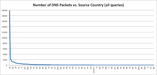
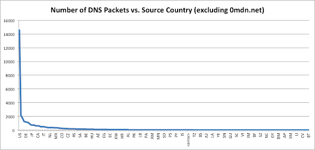
The <error> field means the MaxMind GeoLite database did not have an entry for the particular IP address.

The large numbers for the US is likely due to the US-centric nature of many of the domains I bitsquatted, such as fbcdn.net, and the fact that the US just has considerably more IP allocations than other countries. The extensive world coverage of bitsquatting queries is really quite amazing; there are queries from 192 of the 250 countries in the MaxMind database.

Bitsquatting PCAP Analysis Part 3: Bit-error distribution

This is the third post in a multi-post series. The previous post is here.

Which bits are more likely to be affected by bit-errors? What does the bit-error distribution look like?  In this blog post, I will attempt to answer those questions by looking at bit-errors in the requested record type field of DNS queries.

This post actually raises more questions than it answers: the bit-errors of the record type field are not distributed uniformly (the distribution one would expect from a random process), but instead mainly occur in bit 6 of the requested record type. I don't know why this is the case. I also don't know if this is only true for the record type field, or if this extends to the query name field as well. If you have any good suggestions, please contact me.

Bit-errors in the requested record type: A records

Astute readers will have noticed that in the previous post I didn't describe some of the top 15 requested record types. As a refresher, lets take another look at the top 15 most requested record types:

Rank	Query Count	Record Type
1	550892	a
2	509605	aaaa
3	358926	mx
4	26829	any
5	25039	soa
6	7729	cname
7	4835	513
8	4728	ns
9	2597	txt
10	1148	srv
11	698	1025
12	232	257
13	222	a6
14	143	ptr
15	138	spf

The 7th most popular record type is 513. Type 513 is not mentioned in the Wikipedia list of record types, and it is not in Wireshark's record type list. Why are there 4835 requests for an undefined record type?

The answer is clearer when we look at 513 in binary (zero-extended to 16 bits):

0000 0010 0000 0001

This value is only one bit away from 1, the A record request type. Other requested record types in the top 15 share this similarity: type 1025 and type 257 are both one bit away from type 1. In the full query types table there are other requests with this property, such as requests for type 65, 2049, 16385.

The requested record types one bit away from type 1, including binary representation and how often they were requested, are represented below:

Bit Flipped	Binary Value	RR Type	Count	Unique Count	Note
0	1000 0000 0000 0001	32769	0	0
1	0100 0000 0000 0001	16385	5	2
2	0010 0000 0000 0001	8193	0	0
3	0001 0000 0000 0001	4097	0	0
4	0000 1000 0000 0001	2049	22	7
5	0000 0100 0000 0001	1025	698	25
6	0000 0010 0000 0001	513	4835	142
7	0000 0001 0000 0001	257	232	50
8	0000 0000 1000 0001	129	0	0
9	0000 0000 0100 0001	65	128	37
10	0000 0000 0010 0001	33			overlaps SRV
11	0000 0000 0001 0001	17	2	1	overlaps RP
12	0000 0000 0000 1001	9	0	0	overlaps MR
13	0000 0000 0000 0101	5			overlaps CNAME
14	0000 0000 0000 0011	3	0	0	overlaps MD
15	0000 0000 0000 0000	0	2	1

Note: some entries are blank due to overlap with other popular record types. Unpopular/deprecated record types, such as RP, were included in the count for bit errors. All query type overlaps are noted in the notes column.

The count column is how often record type was requested. The unique count column is how often each record type was requested from a unique source IP. This was done to minimize the effect of one bit-error repeatedly manifesting itself via many repeated requests.

A visualization of the unique count column:

To obtain the unique count column, first we must get all the unique (source IP, query type) pairs (and disregard any queries for 0mdn.net):

$ tshark -n -r completelog.pcap -R '!(dns.qry.name contains 0mdn.net)' -o column.format:'"SOURCE", "%s", "QTYPE", "%Cus:dns.qry.type"' | sort -u > analysis/src_and_qtype.txt

After getting the (source IP, query type) pairs, a bash for loop can show us how many unique source IPs requested a certain record type.

$ for qt in 32769 16385 8193 4097 2049 1025 513 257 129 65 SRV RP MR CNAME MD unused; do echo "$qt:" `grep -i " $qt$" analysis/src_and_qtype.txt | wc -l`; done
32769: 0
16385: 2
8193: 0
4097: 0
2049: 7
1025: 25
513: 142
257: 50
129: 0
65: 37
SRV: 80
RP: 1
MR: 0
CNAME: 635
MD: 0
unused: 1

Counting only record requests by unique source IP address shows that the same error-prone query is repeated many times from the same source, but the overall distribution stays the same.

There has been much speculation about bit-error distribution and if any bits are more likely to be affected. Judging by bit-errors of the query type field some bits are considerably more likely to be affected: bit 6 accounts for the vast majority of bit-errors, with the error rate dropping sharply with distance from bit 6. This distribution is evident in the query type field; I have not verified if it still holds in the query name field.

I don't know why the distribution is as skewed as it is. Maybe the distribution is an artifact of the query type field and typical allocation alignments? Other thoughts and ideas are welcome.

Bit-errors in the requested record type: AAAA records

There are nearly as many AAAA record requests as there are A record requests. Do bit-errors of AAAA requests exhibit the same distribution?

Bit Flipped	Binary Value	Value	Count	Unique Count	Note
0	1000 0000 0001 1100	32796	0	0
1	0100 0000 0001 1100	16412	0	0
2	0010 0000 0001 1100	8220	0	0
3	0001 0000 0001 1100	4124	0	0
4	0000 1000 0001 1100	2076	0	0
5	0000 0100 0001 1100	1052	0	0
6	0000 0010 0001 1100	540	4	1
7	0000 0001 0001 1100	284	4	1
8	0000 0000 1001 1100	156	0	0
9	0000 0000 0101 1100	92	0	0
10	0000 0000 0011 1100	60	0	0
11	0000 0000 0000 1100	12			overlaps PTR
12	0000 0000 0001 0100	20	0	0
13	0000 0000 0001 1000	24	0	0
14	0000 0000 0001 1110	30	0	0
15	0000 0000 0001 1101	29	0	0

Despite there being a nearly identical number of queries of reach record types (when excluding queries for 0mdn.net), there are almost no bit-errors for AAAA record queries. The errors that do exist though correspond to errors in bit 6 and bit 7. Some of the discrepancy between the amount of bit errors in A and AAAA queries can be explained since there are simply fewer sources of AAAA queries:

$ tshark -n -r completelog.pcap -R '(dns.qry.type == AAAA) and !(dns.qry.name contains 0mdn.net)' -o column.format:'"SOURCE", "%s"' | sort -u > analysis/aaaa_sources.txt

$ tshark -n -r completelog.pcap -R '(dns.qry.type == A) and !(dns.qry.name contains 0mdn.net)' -o column.format:'"SOURCE", "%s"' | sort -u > analysis/a_sources.txt

$ wc -l analysis/aaaa_sources.txt analysis/a_sources.txt
    7206 analysis/aaaa_sources.txt
   29833 analysis/a_sources.txt

There are only ~24% as many sources of AAAA requests as there are of A requests. Still, this would only account for ~76% of the difference in error rate.

Conclusion

The bit-error distribution, at least with respect to the requested record type field, is not uniform. It is centered at bit 6 and sharply falls off with distance from bit 6. I don't have an explanation as to why, but I suspect might have to do with packet alignment in memory. Other possibilities include errant networking equipment or software somewhere on the Internet. Any ideas and suggestions, especially testable ones, are most welcome.

There are also more bit-errors in A records requests than AAAA record requests. The fact that there are fewer sources of AAAA records accounts for a part of this discrepancy, but does not completely eliminate it.

If you have any insight, please contact me.

Update:
Part 4 is now up, Bitsquatting PCAP Analysis Part 4: Source Country Distribution.

Bitsquatting PCAP Analysis Part 2: Query Types, IPv6

This is the second post in a multi-part series. The previous post is here.

In this installment of Bitsquatting PCAP analysis we will make an educated guess about the prevalence of IPv6 on the Internet, which services DNS is used for, and identify some mysteries in the bitsquatting PCAPs.

All of this information is going to come from just one field: the requested record type of each DNS query.

Background

First, some background on DNS record types. DNS is essentially a distributed hierarchical database. Values are retrieved by specifying a location and a record type. The location is a fully qualified domain name. The record type is one of several defined record types. The most commonly requested record type is A, which means IPv4 address. When you are using IPv4 and translate www.google.com to an IP address,  you are retrieving the A record for www.google.com.

The dig command is used to manually query for DNS records. The following command will retrieve the A record for www.google.com:

$ dig +short www.google.com a
173.194.75.99
173.194.75.147
173.194.75.104
173.194.75.103
173.194.75.105
173.194.75.106

The above command says: ask my local name server (usually specified in /etc/resolv.conf) for the A record for www.google.com. And output the result in short form. Note: the IP addresses returned for you will likely be different. Google attempts to direct you to a physically closer server based on the geo-ip location of the requesting DNS server. This is one part of how most content delivery networks work. More in a future blog post.

One more common record type is AAAA, which is used to retrieve IPv6 addresses. Why is the record type called AAAA? Because IPv4 addresses are 32 bits wide, and IPv6 addresses are 128 bits wide. If A is 32-bit, then AAAA would be 32+32+32+32=128-bit. Interestingly there used to be another record type for retrieving IPv6 addresses, A6, that has since been deprecated. Even if you are using IPv4, you can still retrieve the AAAA record of wwww.google.com:

$ dig +short www.google.com aaaa
2607:f8b0:400c:c01::67

What is DNS used for?

By tallying the frequency of requested record types, we can determine the popularity of DNS uses. The requested record type is specified by the query type field of each DNS request. We can retrieve the query type from each packet using tshark. Lets get a list of all requested record types, and how often each record type was requested:

$ tshark -n -r completelog.pcap  -o column.format:'"QTYPE", "%Cus:dns.qry.type"' | tr '[:upper:]' '[:lower:]' | sort | uniq -c | sort -rn > analysis/all_qtypes.txt

The full record type frequency table is available:  (all_qtypes.txt, 408B, text).

The table below shows the top 15 requested record types. Amazingly, the most requested DNS record type is IPv6 address resolution! Considering that other places measure IPv6 DNS traffic at only 15% of web traffic, something is definitely amiss. More on this after the discussion of DNS use.

Rank	Query Count	Record Type
1	2050660	aaaa
2	1132372	a
3	359779	mx
4	47335	a6
5	38404	any
6	25954	soa
7	8155	cname
8	5130	ns
9	4835	513
10	2622	txt
11	1149	srv
12	698	1025
13	232	257
14	144	ptr
15	141	spf

Name resolution is by far the most popular use of DNS. Name resolution is responsible for the first, second, fourth, and seventh most frequently requested record types. Amazingly there is a very high frequency of deprecated A6 records. Can there really be that many old BIND servers out there?

The second most popular use of DNS is for email related services. The third most requested record type is MX, which is used for determining the incoming mail servers for a domain. MX records can be viewed from the command line as well:

$ dig +short gmail.com mx
10 alt1.gmail-smtp-in.l.google.com.
30 alt3.gmail-smtp-in.l.google.com.
5 gmail-smtp-in.l.google.com.
20 alt2.gmail-smtp-in.l.google.com.
40 alt4.gmail-smtp-in.l.google.com.

Along with MX, the other records commonly used for email are TXT (to hold SPF and DKIM data) which is the tenth most frequently requested, and SPF (used for SPF data) which is the fifteenth most frequent.

The fifth, sixth, and eighth most frequently record types are used all used for DNS infrastructure purposes. The ANY record type simply retrieves all available records, the SOA record type specifies who is the primary source for information about the domain, and the NS type specifies nameservers that can be used to answer queries about the domain.

The next most commonly requested record type, SRV, is used for custom protocol related records. In practice, most SRV queries are used to retrieve information for Jabber/XMPP and other messaging services, including VoIP/Videoconferencing services.

Finally PTR records are used for reverse DNS lookups. A reverse lookup is performed when you want to map an IP address to a domain name. This is one of the few (maybe the only?) time when you will encounter the .arpa TLD. ARPA originally stood for the Advanced Research Projects Agency, the US Government agency that funded the creation of the Internet. These days .arpa has been backronymed to Address and Routing Parameter Area, and what used to be ARPA is now DARPA.

To request a PTR records for an IPv4 address, the octets of the IP are reversed, and .in-addr.arpa is appended. This is because IP addresses are hierarchical from left to right but DNS is hierarchical from right to left. For example, to see what domain 173.194.75.99 (one of the IPs for  www.google.com) corresponds to, we would use the following command:

$ dig +short 99.75.194.173.in-addr.arpa ptr
ve-in-f99.1e100.net.

The returned domain is not www.google.com, but this is due to Google's infrastructure. There is a clever easter egg in the domain: 1e100 means 1.0 × 10¹⁰⁰, which is one googol.

What can we learn about the prevalence of IPv6?

Before we jump to conclusions about IPv6, we should remember that there are outliers in the bitsquatting PCAPs. If you recall from the previous post, there were numerous queries for 0mdn.net because that domain was an authoritative name server. Queries for 0mdn.net might be affecting the record type distribution. Lets filter out these queries:

$ tshark -n -r completelog.pcap -R '!(dns.qry.name contains 0mdn.net)' -o column.format:'"QTYPE", "%Cus:dns.qry.type"' | tr '[:upper:]' '[:lower:]' | sort | uniq -c | sort -rn > analysis/nomdn_qtypes.txt

The full list of record types and their frequencies is available: (nomdn_qtypes.txt, 379B, text).

This command works using the -R option of tshark. The -R option specifies a wireshark display filter that is applied when reading PCAPs. The filter of !(dns.qry.name contains 0mdn.net) will match all packets where the query name field does not contain 0mdn.net. Lets examine the new results:

Rank	Query Count	Record Type
1	550892	a
2	509605	aaaa
3	358926	mx
4	26829	any
5	25039	soa
6	7729	cname
7	4835	513
8	4728	ns
9	2597	txt
10	1148	srv
11	698	1025
12	232	257
13	222	a6
14	143	ptr
15	138	spf

The new table is a much different picture with regards to IPv6, but there is still a large amount of AAAA record requests.

Lesson Learned: There are enough AAAA record requests to indicate IPv6 connectivity is important. If you are attempting to re-do the bitsquatting experiment, have IPv6 connectivity and answer AAAA requests!

What is the nature of IPv6 traffic (AAAA record requests)?

Why were there so many AAAA record requests for the authoritative nameservers, and how do these compare to other domains? Lets use tshark to retrieve all AAAA record requests, and which domain was the request was for:

$ tshark -n -r completelog.pcap -R '(dns.qry.type == AAAA)' -o column.format:'"QTYPE", "%Cus:dns.qry.name"' | tr '[:upper:]' '[:lower:]' | sort | uniq -c | sort -rn > analysis/AAAA_queries.txt

The full list of AAAA query frequencies is available: (AAAA_queries.txt, 17KB, text).

AAAA Queries	Domain
794921	ns2.0mdn.net
774496	ns1.0mdn.net
77181	static.ak.dbcdn.net
77053	support.doublechick.net
66595	gmaml.com
58634	g.mic2osoft.com
28107	s0.0mdn.net
16327	www.amazgn.com
13401	mail.gmaml.com
6367	www.micro3oft.com
5678	amazgn.com
4924	www.mic2osoft.com
4789	www.eicrosoft.com
4578	pop.gmaml.com
4346	static.ak.fbgdn.net

The two authoritative name servers receive the most AAAA requests, but there are other domains with numerous IPv6 lookups. Maybe these domains are just popular?

Ratio of IPv4 to IPv6 address lookups

The ratio of IPv4 address resolutions to IPv6 address resolutions will show the proportion of IPv6 traffic for each domain. This measurement should completely disregard popularity, as it uses ratios instead of absolute numbers. My hypothesis was that the ratios should be approximately the same for all domains, as none of the domains I bitsquatted were IPv6 related. Lets calculate the ratios. 

Step 1: Calculate A record frequency

The following command will tabulate the frequency of A record requests for each domain:

$ tshark -n -r completelog.pcap -R '(dns.qry.type == A)' -o column.format:'"QTYPE", "%Cus:dns.qry.name"' | tr '[:upper:]' '[:lower:]' | sort | uniq -c | sort -rn > analysis/A_queries.txt

The full list of A query frequencies is available: (A_queries.txt, 99KB, text).

Step 2: Massage Data

The following commands will prepare both the A record frequency and AAAA record frequency tables to be joined on the domain name field.

$ sort -f -k2 analysis/A_queries.txt  > a_q_for_join.txt
$ sort -f -k2 analysis/AAAA_queries.txt  > aaaa_q_for_join.txt

Step 3: Calculate the ratio of A to AAAA record requests

Amazingly, the POSIX standard specifies a relational join command that operates on specially delimited text files. The join command below will join the first file on the second field (-1 2), with the second file also on the second field (-2 2). The second field of both files is the domain name. The output of join is then piped to awk to calculate the ratio of A to AAAA record requests.

$ join -1 2 -2 2 a_q_for_join.txt aaaa_q_for_join.txt | awk '{printf "%d\t%2.2f\t%s\n", $2+$3, $2/$3, $1}' | sort -rn >analysis/ratio_of_a_to_aaaa.txt

The full list of A:AAAA ratios is available: (ratio_of_a_to_aaaa.txt, 18KB, text).

Total Query Count	A to AAAA Query Ratio	Domain
1095763	0.41	ns1.0mdn.net
1072642	0.35	ns2.0mdn.net
93208	0.40	gmaml.com
80862	0.05	static.ak.dbcdn.net
77147	0.00	support.doublechick.net
70140	4.23	mail.gmaml.com
59500	0.01	g.mic2osoft.com
53969	2.31	www.amazgn.com
43270	6.62	amazgn.com
28694	0.02	s0.0mdn.net
20575	8.63	micro3oft.com
13585	9.32	miarosoft.com
12175	0.91	www.micro3oft.com
10762	1.19	www.mic2osoft.com
9032	26.62	u2s.micro3oft.com

Different domains exhibit a wildly different ratio of IPv4 to IPv6 lookups! Some actually have more IPv6 resolutions than IPv4 resolutions. The mystery is, why is this the case?

Conclusion

IPv6 connectivity is important. When removing outliers, there were almost as many IPv6 resolution requests as IPv4 requests. When investigating in more detail, some domains actually receive more IPv6 resolution requests than IPv4 resolution requests. I do not know why. If you have suggestions, please contact me.

Update:
Part 3 is now up, Bitsquatting PCAP Analysis Part 3: Bit-error distribution.

Bitsquatting PCAP Analysis Part 1: Analyzing PCAPs using Unix command line tools

This blog post was originally going to be about domain name distribution in the bitsquatting PCAPs, but I found a problem with my first analysis. The problem has been turned into an opportunity, and now this blog post is about domain name distribution in the bitsquatting PCAPs, and a tutorial on how to determine the distribution yourself!

This blog post/tutorial will follow the process I used to answer the following questions:

• How many unique domains appear in queries directed at the bitsquatting nameserver? Answer: 4271.
• What is the frequency distribution of queried domains? Answer: long tail; percentages here.

Prerequisites

A basic familiarity with Unix is assumed throughout this tutorial. While all the commands listed were run on Mac OS X, any sufficiently Unix-y environment should work.

To do the analysis we are going to install some extra software. We will need the following:

• wireshark (specifically, the tshark and mergecap utilities) to dissect packet captures
• the GNU version of coreutils (for ls -v)
• 7zip to decompress the compressed DNS packet captures
• and wget because I hate remembering to use "curl -O" to download via the command line.

All the prerequisites should be easily available with your favorite package manager. Since all command examples in this tutorial were run on Mac OS X, I installed the prerequisites via homebrew:

# brew install coreutils
# brew install wireshark
# brew install p7zip
# brew install wget

Downloading and Extracting the Data

The first step of analysis is to get the data. Lets download and extract the Bitsquatting PCAPs:

$ wget http://dinaburg.org/data/dnslogs.tar.7z
$ 7z x dnslogs.tar.7z
$ tar xvf dnslogs.tar
$ rm dnslogs.tar dnslogs.tar.7z

Numerous files named dnslog, dnslog1, dnslog2, etc. should now be in your working directory. These files contain packet captures (PCAPs) of DNS traffic.

The tcpdump utility is the most basic way to analyze PCAP contents. Lets take a look to see what the logs contain:

$ tcpdump -n -v -r dnslog

All of the output should be details about DNS queries. The output format is described in detail on the tcpdump man page. This tutorial is not about tcpdump, I included this step since it is a very good idea to investigate any unknown PCAPs with tcpdump and look for oddities before opening them in more complex tools. Opening files from unknown sources in wireshark can be dangerous. Even though it wont be further referenced in this blog post, the tcpdump utility is extremely handy; I highly recommend reading some tcpdump tutorials for background knowledge.

Combining PCAPs

The PCAPs are cumbersome to work with since they are split into several files. To make analysis easier, lets re-assemble all the disparate PCAPs into a single file. There is a tool called mergecap that comes with wireshark that is made exactly for this purpose.

$ mergecap -a -w completelog.pcap `gls -1v`

The above command will use mergecap in append mode (-a), and save the result into completelog.pcap. Append mode instructs mergecap to simply concatenate the files with correct headers, otherwise mergecap will use packet timestamps to create combined file. The files to merge are given by "gls -1v". Note: gls is GNU ls, it is used because the default ls on Mac OS X does not have a numeric sort option. If you are using Linux just use "ls -1v" in your command line. 

Initial Analysis

Now that we have a merged PCAP, lets do some analysis. To review, the two questions we will answer in this blog post are:

• How many unique domains appear in queries directed at the bitsquatting nameserver?
• What is the frequency distribution of queried domains ?

The answers to both of these questions depend on extracting the query name from every incoming DNS query. Luckily we will not need two write any PCAP reading code; there are many great projects specifically meant for dissecting PCAPs. In this post, we will be using using tshark, the text-only part of the wireshark network traffic analyzer as our PCAP dissector.

The following tshark command will display the query name field of every DNS query in completelog.pcap:

$ tshark -n -r completelog.pcap  -o column.format:'"QNAME", "%Cus:dns.qry.name"'

The above command instructs tshark to not attempt DNS resolution (-n), to read from completelog.pcap as the packet source (-r), and to override the default output format to be the dns.qry.name field of the packet (-o).

The tshark utility supports many output formats. The column.c file in the wireshark source specifies allowed formats. It is my understanding that the custom format specifier (%Cus) can accept any protocol filter field. The wireshark Display Filter DNS Protocol reference specifies all filter fields for the DNS protocol.

If you ran the command you will notice it takes a long time to finish. Its best to pick a small subset of the data first and ensure there are no problems before working with the full set. Lets verify that it is possible to count domain frequency in the first 1000 queries:

$ tshark -n -r completelog.pcap  -o column.format:'"QNAME", "%Cus:dns.qry.name"' | head -n 1000 | sort | uniq -c | sort -rn
 183 ns1.0mdn.net
 171 ns2.0mdn.net
 129 eicrosoft.com
 108 micro3oft.com
  85 mic2osoft.com
  65 static.ak.fbgdn.net
  44 www.micro3oft.com
  38 iicrosoft.com
  32 gmaml.com
  24 www.mic2osoft.com
  20 www.miarosoft.com
  19 www.amazgn.com
  14 profile.ak.fjcdn.net
  13 forum.micro3oft.com
  12 mscrl.eicrosoft.com
  12 0mdn.net
  11 amazgn.com
   8 profile.ak.fbgdn.net
   8 aeazon.com
   2 www.gmaml.com
   2 www.eicrosoft.com

It turns out there are casing issues with the query name field: micro3oft.com and MICRO3OFT.COM are counted as different domains although they are semantically the same. Domain resolution is case-insensitive, but query name case can matter. For instance, 0x20 encoding uses query name casing to increase DNS query entropy. Increasing query entropy makes DNS forgery attacks more difficult. More details can be found in the 0x20 encoding paper.

Since we are interested in only the semantic meaning of domains, they should all be converted to lower case before frequency counting. This can be done by piping the names through tr. The new command line should only output lowercased domains:

$ tshark -n -r completelog.pcap  -o column.format:'"QNAME", "%Cus:dns.qry.name"' | head -n 1000 | tr '[:upper:]' '[:lower:]' | sort | uniq -c | sort -rn
 183 ns1.0mdn.net
 171 ns2.0mdn.net
 129 eicrosoft.com
 108 micro3oft.com
  85 mic2osoft.com
  65 static.ak.fbgdn.net
  44 www.micro3oft.com
  38 iicrosoft.com
  32 gmaml.com
  24 www.mic2osoft.com
  20 www.miarosoft.com
  19 www.amazgn.com
  14 profile.ak.fjcdn.net
  13 forum.micro3oft.com
  12 mscrl.eicrosoft.com
  12 0mdn.net
  11 amazgn.com
   8 profile.ak.fbgdn.net
   8 aeazon.com
   2 www.gmaml.com
   2 www.eicrosoft.com

Our problem is solved. Lets create a directory for our analysis outputs and count the domain frequency in the full data set:

$ mkdir analysis
$ tshark -n -r completelog.pcap  -o column.format:'"QNAME", "%Cus:dns.qry.name"' | tr '[:upper:]' '[:lower:]' | sort | uniq -c | sort -rn > analysis/requested_domains.txt

The full frequency count can be viewed here: (requested_domains.txt, 117KB, text).

Now we can finally answer our first question: How many unique domains appear in queries directed at the bitsquatting name server? Since the resulting file has one domain per line, the line count will be the number of unique domains:

$ wc -l analysis/requested_domains.txt
  4271 analysis/requested_domains.txt

There was a total of 4271 unique requested domains. 

Removing Outliers

Lets try to get a feel for the distribution of domains in the query name field. First, lets look at the most frequently requested domains:

$ head -n 10 analysis/requested_domains.txt 
1124949 ns1.0mdn.net
1101708 ns2.0mdn.net
184405 gmaml.com
142283 support.doublechick.net
80865 static.ak.dbcdn.net
78839 miarosoft.com
70174 mail.gmaml.com
59500 g.mic2osoft.com
57514 microsmft.com
54125 www.amazgn.com

The left column is the number of times the domain appeared in the query name field, and the right column is the domain. 

The domains ns1.0mdn.net and ns2.0mdn.net are outliers, they are by far the most frequently requested. These domains were the authoritative name servers for my bitsquatting domains. The high frequency of queries for these domains has nothing to do with their popularity and has everything to do with their authoritative name server status. Including them in the top 10 count would be improper. The new top ten most frequently queried domains, with authoritative servers excluded are:

184405 gmaml.com
142283 support.doublechick.net
80865 static.ak.dbcdn.net
78839 miarosoft.com
70174 mail.gmaml.com
59500 g.mic2osoft.com
57514 microsmft.com
54125 www.amazgn.com
45866 amazgn.com
32021 mssupport.micrgsoft.com

Calculating Percentages

Raw query numbers are interesting, but to better comprehend query name frequency the percentage of total queries is a better measurement. To calculate the percentages we first need to calculate the total number of queries excluding queries for authoritative name servers. The following awk script will add all values in the the query count column (the first column) of requested_domains.txt, excluding the first two rows (the query counts for the authoritative name servers):

$ awk 'NR > 2 {sum+=$1} END {print sum}' < analysis/requested_domains.txt
1451284

Using the total number of queries we can write another awk script to convert query frequencies into percentages. Lets look at the percentage of queries represented by each of the top 10 most frequently queried domains:

$ awk 'NR > 2 {printf "%2.2f %s\n", $1/1451284*100, $2}' < analysis/requested_domains.txt | head -n 10
12.71 gmaml.com
9.80 support.doublechick.net
5.57 static.ak.dbcdn.net
5.43 miarosoft.com
4.84 mail.gmaml.com
4.10 g.mic2osoft.com
3.96 microsmft.com
3.73 www.amazgn.com
3.16 amazgn.com
2.21 mssupport.micrgsoft.com

The full percentages can be downloaded here: (requested_domain_percentage.txt, 117KB, text).

We have now answered the second question: What is the frequency distribution of queried domains? The domain frequency distribution is a superb example of a long tail.

Update:
Part 2 is now up, Bitsquatting PCAP Analysis Part 2: Query Types, IPv6.