This is part 4 of a multipart series, the previous post is Bitsquatting PCAP Analysis Part 3: Bit-error distribution.
This blog post will examine the source country distribution of packets in the bitsquatting PCAPs. To map a source IP address to a physical location, we will use MaxMind's free GeoLite Data (available at http://dev.maxmind.com/geoip/geolite) as the data source, and write a quick Python script using pygeoip to do the IP-to-location translation.
First, lets download and decompress the free GeoLite City Database provided by MaxMind:
Next, we will install pygeoip. The installation procedures for Python packages vary, but its likely that pygeoip can be installed by setuptools:
The pygeoip page on github provides all the necessary usage examples to create an IP-to-country script. My script, which reads in IPv4 addresses line-by-line on from a file (or stdin) and outputs an "ip:country:city" mapping is available here: ip_to_city_country.py.
The example usage:
The first step to mapping source country frequency is to identify source address frequency. While the source address frequency is only an intermediate step to gather source country distribution, it is very handy for a manual analysis of where queries are coming from.
A read-filter can be applied to get the source IPs with the 0mdn.net outliers removed:
The results for the frequency of all source IPs (ips_all.txt, 848KB, text) and only IPs not requesting 0mdn.net (ips_nomdn.txt, 740KB, text) are available for download.
These intermediate results show how many packets were received from each IP. The list is interesting in its own right. The top few results are an unresponsive IP in Poland, IPs with PTR records pointing to subdomains of rscott.org (possibly in related to http://rscott.org/dns/ ?), an open-recursive namserver at a Russian ISP, a resolver for LeaseWeb, and an MTA for WindStream Communications. Feel free to investigate more on your own.
To find the frequency of source countries, each address will be mapped to its origin country. Only unique addresses, not how many packets were received from each address, will be counted for the distribution. Some shell commands and the ip_to_city_country.py script will identify the source countries. In the commands below, gcut, the GNU version of cut is used since the default cut on Mac OS X cannot handle non-ASCII characters.
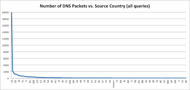
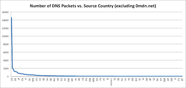
The all country frequency table (all_country_frequency.txt, 1.5KB, text) and the frequency table sans requests for 0mdn.net (nomdn_country_frequency.txt, 1.5KB, text) have very similar distributions, only the magnitude changes. This is easier to see in graph form:
The <error> field means the MaxMind GeoLite database did not have an entry for the particular IP address.
The large numbers for the US is likely due to the US-centric nature of many of the domains I bitsquatted, such as fbcdn.net, and the fact that the US just has considerably more IP allocations than other countries. The extensive world coverage of bitsquatting queries is really quite amazing; there are queries from 192 of the 250 countries in the MaxMind database.
This blog post will examine the source country distribution of packets in the bitsquatting PCAPs. To map a source IP address to a physical location, we will use MaxMind's free GeoLite Data (available at http://dev.maxmind.com/geoip/geolite) as the data source, and write a quick Python script using pygeoip to do the IP-to-location translation.
IP to Location Translation
First, lets download and decompress the free GeoLite City Database provided by MaxMind:
$ wget http://geolite.maxmind.com/download/geoip/database/GeoLiteCity.dat.gz
$ gunzip GeoLiteCity.dat.gz
Next, we will install pygeoip. The installation procedures for Python packages vary, but its likely that pygeoip can be installed by setuptools:
# easy_install pygeoip
The pygeoip page on github provides all the necessary usage examples to create an IP-to-country script. My script, which reads in IPv4 addresses line-by-line on from a file (or stdin) and outputs an "ip:country:city" mapping is available here: ip_to_city_country.py.
The example usage:
$ ./ip_to_city_country.py --help
usage: ip_to_city_country.py [-h] [-d GEOIPDB] [ipfile]

Show city and country of IP addresses using MaxMind GeoIP Database

positional arguments:
  ipfile      a file from which to read IP addresses (default: stdin)

optional arguments:
  -h, --help  show this help message and exit
  -d GEOIPDB  Path to the GeoIPCity database (default: GeoLiteCity.dat)


$ echo '8.8.8.8' | ./ip_to_city_country.py
8.8.8.8:US:Mountain View
Source Address Frequency
The first step to mapping source country frequency is to identify source address frequency. While the source address frequency is only an intermediate step to gather source country distribution, it is very handy for a manual analysis of where queries are coming from.
$ tshark -n -r completelog.pcap -o column.format:'"SOURCE", "%s"' | sort | uniq -c | sort -rn > analysis/ips_all.txt
A read-filter can be applied to get the source IPs with the 0mdn.net outliers removed:
$ tshark -n -r completelog.pcap -R '!(dns.qry.name contains 0mdn.net)' -o column.format:'"SOURCE", "%s"' | sort | uniq -c | sort -rn > analysis/ips_nomdn.txt
The results for the frequency of all source IPs (ips_all.txt, 848KB, text) and only IPs not requesting 0mdn.net (ips_nomdn.txt, 740KB, text) are available for download.
These intermediate results show how many packets were received from each IP. The list is interesting in its own right. The top few results are an unresponsive IP in Poland, IPs with PTR records pointing to subdomains of rscott.org (possibly in related to http://rscott.org/dns/ ?), an open-recursive namserver at a Russian ISP, a resolver for LeaseWeb, and an MTA for WindStream Communications. Feel free to investigate more on your own.
Source Country Frequency
To find the frequency of source countries, each address will be mapped to its origin country. Only unique addresses, not how many packets were received from each address, will be counted for the distribution. Some shell commands and the ip_to_city_country.py script will identify the source countries. In the commands below, gcut, the GNU version of cut is used since the default cut on Mac OS X cannot handle non-ASCII characters.
$ awk '{print $2}' analysis/ips_all.txt | ./ip_to_city_country.py > analysis/ip_all_location_mapping.txt

$ gcut -f 2 -d ':' analysis/ip_all_location_mapping.txt | sort | uniq -c | sort -rn  > analysis/all_country_frequency.txt

$ awk '{print $2}' analysis/ips_nomdn.txt | ./ip_to_city_country.py > analysis/ip_nomdn_location_mapping.txt

$ gcut -f 2 -d ':' analysis/ip_nomdn_location_mapping.txt | sort | uniq -c | sort -rn > analysis/nomdn_country_frequency.txt
The all country frequency table (all_country_frequency.txt, 1.5KB, text) and the frequency table sans requests for 0mdn.net (nomdn_country_frequency.txt, 1.5KB, text) have very similar distributions, only the magnitude changes. This is easier to see in graph form:
The <error> field means the MaxMind GeoLite database did not have an entry for the particular IP address.
The large numbers for the US is likely due to the US-centric nature of many of the domains I bitsquatted, such as fbcdn.net, and the fact that the US just has considerably more IP allocations than other countries. The extensive world coverage of bitsquatting queries is really quite amazing; there are queries from 192 of the 250 countries in the MaxMind database.


